How I Build a Bear / Base / Bull Model

When I open a company, I do not start by asking how high the stock can go. I start with a much more annoying question:

What actually drives per-share value here?

If I get that wrong, I can build an absolutely gorgeous spreadsheet that tells me nothing useful. If I get it right, most of what comes next is just arithmetic.

Before the cases, I figure out what kind of model this needs

Before touching bear/base/bull, I need to know what kind of model I am actually building. Three questions usually tell me how much of the financial statements I need to rebuild.

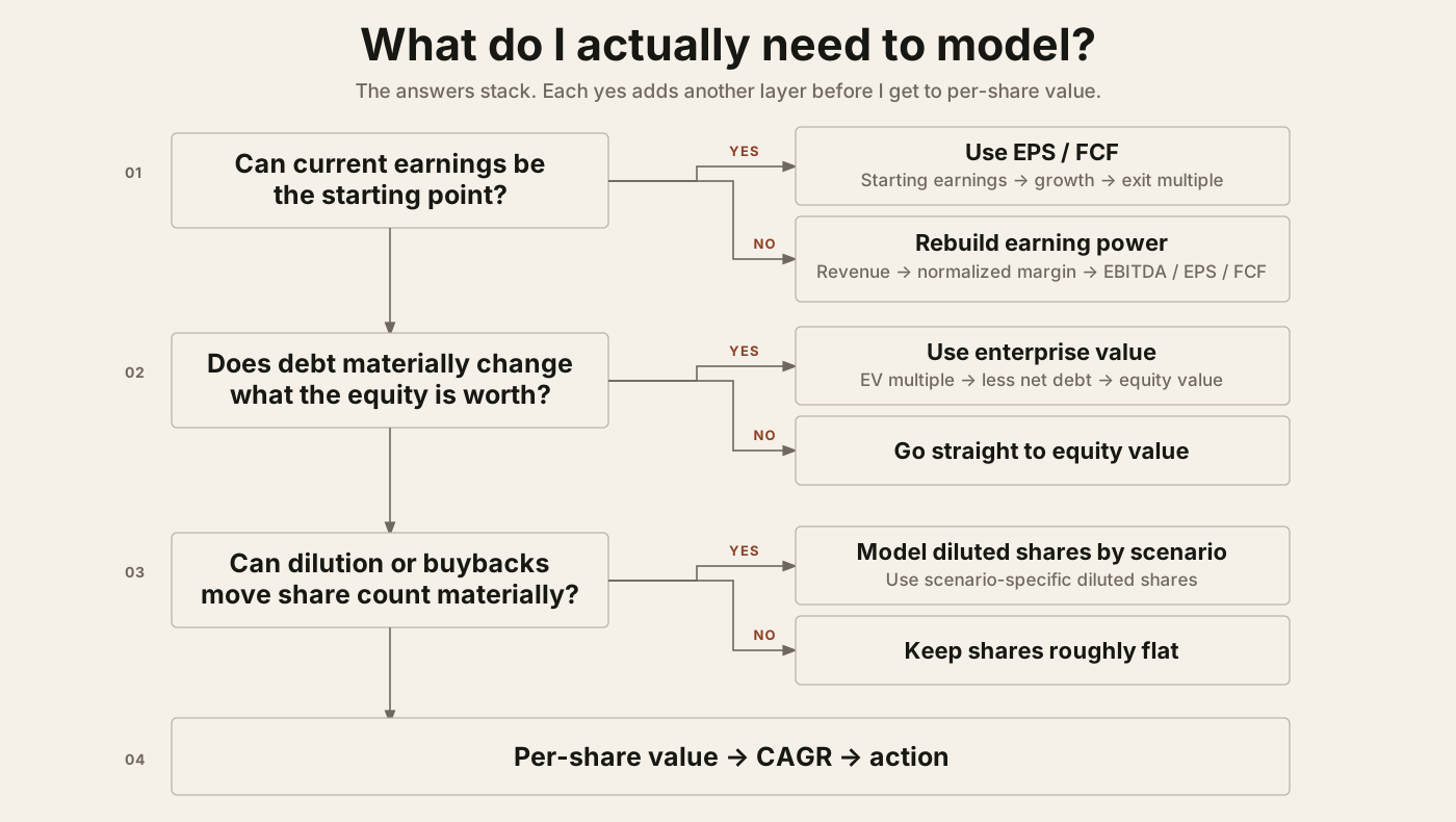
For the two examples below, the paths are simple:

• MSFT: yes → no → no. I can start with EPS, and neither leverage nor dilution changes the structure much.
• BRBR: no → yes → yes. I need to rebuild earnings power, subtract debt, and model the share count.

Before I calculate anything, I also label every number as one of four things:

Input type	What it is	Where it comes from
Reported fact	Revenue, EPS, debt, shares, margins	Company filing / earnings release
Market input	Share price	Live market price when I run the model
External estimate	Consensus EPS, revenue, etc.	Dated analyst-consensus source
Underwriting assumption	Growth rate, terminal multiple, normalized margin	My judgment, supported by the evidence above

The distinction is simple and really important: facts get sourced. Assumptions get defended. A terminal multiple does not become a fact because I put it in a tidy table.

---

Example 1 — Microsoft: EPS growth + terminal P/E

Microsoft is the easy example, structurally at least.

Current earnings are useful, the balance sheet is not the main risk to equity value, and the question is mostly:

How fast can EPS compound, and what multiple is reasonable five years from the starting point?

Step 1 — find a cleaner starting EPS

For this MSFT model:

Starting EPS = $17.28

Microsoft reported FY2026 diluted GAAP EPS of $17.95, but its full-year release also shows that net gains from the OpenAI investment added $0.67 per share. Microsoft therefore reports $17.28 of OpenAI-adjusted EPS.

For an operating valuation model, I use the $17.28 figure.

That does not make $17.28 some magical “true EPS.” It is still a company-defined adjusted number, and Q4 had other discrete items too. I just think it is a cleaner operating anchor than pretending an investment gain is recurring earnings forever.

Source: Microsoft FY2026 Q4 / full-year earnings release

Step 2 — set the horizon

For Microsoft:

Horizon = 5 years

Step 3 — build the EPS growth assumptions

The starting facts are strong:

Evidence	Current evidence	What it tells me
FY2026 revenue growth	18%	Microsoft is still growing unusually fast off a huge base
FY2026 operating income growth	21%	Profit grew faster than revenue
FY2026 adjusted EPS growth	22%	Cleaner than the 32% GAAP figure because it removes the OpenAI investment effect
Q4 Azure growth	43%	Azure remains the main growth engine
Q1 FY2027 Azure guide	~45% cc	Near-term commercial momentum is still exceptional
Q1 FY2027 total revenue guide	16%–17%	The consolidated growth rate is not collapsing yet
Microsoft Cloud gross margin	65% Q4 / 66% FY26	The AI build is expensive; FY25 was 69%
Q1 FY2027 capex guide	>$50B	The capital intensity is still increasing
Diluted share count	7.453B vs. 7.465B	Buybacks provide very little EPS help

Sources: FY2026 earnings release, FY2026 investor metrics, and FY2026 Q4 earnings call / FY2027 outlook.

The shorthand is still:

EPS growth ≈ sustainable revenue growth + operating leverage + share-count effect

My five-year assumptions are:

Scenario	Sustainable revenue growth I am roughly assuming	Margin / share-count contribution	EPS growth assumption	Why
Bear	~8%	~1 pt	9%	Azure/AI normalize, mature businesses dominate more of the mix and infrastructure intensity limits margin leverage
Base	~13%	~2 pts	15%	Growth fades from today’s pace, but cloud/AI mix and operating leverage keep EPS compounding around the mid-teens
Bull	~16%	~2 pts	18%	Azure/AI stay unusually strong and monetization catches up with the infrastructure bill without requiring heroic share-count help

The base stays at 15% because the FY2027 starting guide can actually support it. I am definitely not taking FY2026’s 22% adjusted EPS growth and dragging it five years into the future because the number is convenient.

The bear moves to 9% because the downside I actually worry about is much more boring than Microsoft breaking: AI is real, the business keeps growing, and the return on all that infrastructure spend is just less exciting than everyone hoped.

The bull is 18%, not 20%+, because let’s be real, sustaining 18% EPS growth for five years from Microsoft’s current scale is already ridiculous.

Formula:

Future EPS = Starting EPS × (1 + growth rate)^years

Base case:

$17.28 × 1.15^5 = ~$34.76

Step 4 — decide what terminal multiple I can defend

I also reset the terminal multiples.

Scenario	Terminal P/E	Why
Bear	22x	Excellent business, but lower growth plus persistent capital intensity earns real multiple compression
Base	28x	A premium multiple for a high-quality company still compounding earnings around the mid-teens
Bull	32x	Faster growth persists and the market still pays a large quality/growth premium

The old example used 24x / 30x / 34x. I do not want the thesis depending on today’s premium multiple politely waiting for me five years from now.

Step 5 — turn the earnings into a future share price

Future share price = Future EPS × Terminal P/E

MSFT scenario	Future EPS	Terminal P/E	Implied value
Bear	~$26.59	22x	~$585
Base	~$34.76	28x	~$973
Bull	~$39.53	32x	~$1,265

Step 6 — see what each outcome means for the return

Formula:

CAGR = (Future value ÷ Live share price)^(1 ÷ years) - 1

For the dated worked example, use the Sep. 25, 2026 close of $516.17:

Scenario	Implied value	Example 5-year price CAGR
Bear	~$585	~2.5%
Base	~$973	~13.5%
Bull	~$1,265	~19.6%

Dividends are not included in those price CAGRs.

On the living company page, the quote moves and the CAGR moves with it. The operating assumptions do not get to chase the stock around. Otherwise I am just letting price action edit the thesis for me.

Step 7 — work backward into buy bands

The entry framework keeps the same P/E discipline and applies it to the cleaner $17.28 earnings anchor:

Entry level	P/E on $17.28 EPS	Approx. price	Base-case 5Y price CAGR
Starter	26x	~$449	~16.7%
Normal	24.5x	~$423	~18.1%
Aggressive	23x	~$397	~19.6%

Formula:

Entry price = Starting EPS × Entry P/E

Normal band:

$17.28 × 24.5 = $423.36

The entry multiple and terminal multiple are two different jobs. One is what I am willing to pay today. The other is what I assume somebody else pays at the end. Mixing them together is a very easy way to make the model nicer than it deserves to be.

A lot of my actual MSFT buying happened before this exact FY2026 anchor existed, so I am not going back and pretending every old purchase was made with today’s model. The way I handle it now is simpler: use the best defensible anchor I have, ask for a return that is actually worth the risk, and compare Microsoft with the other places the money could go.

---

Example 2 — BellRing: revenue → EBITDA → enterprise value → equity value

BRBR is where the neat EPS model stops being useful.

Current earnings are basically the thing I am trying to normalize, debt absolutely matters to the equity, and the share count has moved enough that hiding it would be convenient in exactly the wrong way.

So the engine is:

Revenue → EBITDA margin → EBITDA → EV/EBITDA → net debt → diluted shares → per-share value

Step 1 — put the starting facts on one page

Before choosing a scenario, I want the dated operating facts on one page.

Reported evidence	FY2025 / FY2026 input	Why I care
FY2026 sales guidance	$2.335B–$2.375B	Gives me the revenue anchor
FY2026 adjusted EBITDA guidance	$275M–$295M	Shows how damaged FY2026 profitability is
Implied FY2026 EBITDA margin	~12%	FY2026 margin starting point
FY2025 sales	$2.317B	Revenue was already around the FY2026 run-rate before the margin collapse
FY2025 adjusted EBITDA	$481.6M	Shows how different normal-ish profitability looked one year earlier
FY2025 EBITDA margin	~20.8%	Useful reference for what the business has actually earned before
Q3 FY2026 net sales growth	+4.2%	Demand slowed, but sales did not collapse
Q3 FY2026 gross margin	28.6% vs. 35.4%	The damage is concentrated in profitability
Premier Protein RTD consumption	+6%	Consumer demand still exists
Premier Protein distribution points	+27%	Distribution is still expanding
Long-term debt	$1.135B	Leverage is large enough to matter to equity value
Cash	$50.4M	Starting point for net debt
Q3 diluted weighted-average shares	116.6M	Starting share-count anchor

Primary sources: BellRing Q3 FY2026 earnings release, Q3 FY2026 10-Q, Q3 supplemental, and BellRing 2025 Annual Report.

One old management framework is useful as a sanity check: before the 2026 margin mess, BellRing talked about 7%–9% annual sales growth and 18%–20% adjusted EBITDA margins over the long run. Useful reference point? Yep. Promise? Absolutely not.

Step 2 — set the horizon

For the long-run BRBR model:

Horizon = 5 years / 2031

Why five years?

Because the thesis needs enough time for three different things to happen:

1. revenue to compound;
2. margins to recover or fail to recover;
3. debt and share count to change.

A one-year model can tell me whether the recovery is starting. It cannot tell me whether the whole equity story actually works.

Step 3 — build the revenue scenarios

I start with the midpoint of FY2026 sales guidance:

($2.335B + $2.375B) ÷ 2 = $2.355B

Then I ask what five years of revenue growth would actually produce each 2031 scenario.

Formula:

Revenue CAGR = (2031 revenue ÷ $2.355B)^(1 ÷ 5) - 1

Scenario	2031 revenue	Implied 5-year revenue CAGR	Why
Bear	$2.40B	~0.4%	Demand basically goes nowhere after 2026; FY2026 category/brand strength fails to translate into growth
Base	$2.90B	~4.3%	The brand keeps growing, but well below the old 7%–9% long-term algorithm
Bull	$3.30B	~7.0%	Revenue gets back to roughly the low end of management’s old long-term algorithm

Same rule as Microsoft: reported growth is evidence. It is not a permission slip to copy-paste the rate into the future.

The base case is deliberately below the old company algorithm because FY2026 gave me a reason to demand a haircut.

Step 4 — build the margin scenarios

This is the core BRBR question.

First calculate the FY2026 guided margin using the midpoints:

$285M EBITDA ÷ $2.355B revenue = ~12.1%

Then compare it with the prior year:

$481.6M EBITDA ÷ $2.3166B revenue = ~20.8%

So I have two real anchors:

• FY2026 guided economics: ~12%
• FY2025 economics: ~20.8%

Management’s old long-term algorithm of 18%–20% gives me another reference point.

That leads to:

Scenario	2031 EBITDA margin	What I am underwriting
Bear	12%	The margin problem is basically structural; five years pass and profitability barely improves
Base	16%	A meaningful recovery, but still well below FY2025 and below the old 18%–20% algorithm
Bull	19%	The business gets back near the old long-term range without assuming a new record margin

That is why base lands at 16%: enough recovery for the thesis to work, but nowhere near a full return to 2025 economics. I do not need perfection. I do need the current mess to be at least partly temporary.

Step 5 — calculate EBITDA

Formula:

EBITDA = Revenue × EBITDA margin

Scenario	Revenue	Margin	EBITDA
Bear	$2.40B	12%	$288M
Base	$2.90B	16%	$464M
Bull	$3.30B	19%	$627M

Base case:

$2.90B × 16% = $464M EBITDA

At this point the operating case is built. Everything after it is the bridge to what one share is worth.

Step 6 — decide what terminal EV/EBITDA each case can justify

These multiples are my assumptions. They do not come from a filing.

I link the multiple to the quality of the business that exists in each scenario rather than giving every case the same valuation.

Scenario	EV/EBITDA	Why
Bear	6x	Low growth, no meaningful margin recovery, heavy leverage: still a distressed-looking business
Base	8x	Partial recovery and decent brand economics, but not enough evidence to underwrite a premium multiple
Bull	10x	Healthy growth, margins near the old long-term range, and a much cleaner balance sheet

The thing I am trying to avoid is letting the bull case win four different ways at once. If I already gave it better revenue, better margins and less debt, a heroic exit multiple on top starts feeling more like wishful thinking than underwriting.

Step 7 — build the debt scenarios

At June 30, 2026:

Long-term debt = $1.135B

Cash = $50.4M

So the starting net-debt anchor is roughly:

$1.135B - $0.050B = ~$1.085B

Now I ask how much deleveraging each scenario requires over five years.

Scenario	2031 net debt	Total reduction from ~$1.085B	Rough annual reduction
Bear	$1.0B	~$85M	~$17M/year
Base	$0.6B	~$485M	~$97M/year
Bull	$0.3B	~$785M	~$157M/year

Can the base and bull debt paths actually happen?

BellRing is asset-light, with capital expenditures historically under 1% of sales, and it generated $260.6M of operating cash flow in FY2025. If margins recover, there is a path to meaningful cash generation.

But none of that deleveraging is automatic. Management can use the cash for buybacks, acquisitions or something else entirely, which is why debt and share count need their own assumptions instead of one hand-wavy ‘capital allocation improves’ line.

Step 8 — build the share-count scenarios

Q3 FY2026 diluted weighted-average shares were 116.6M.

BellRing has also been an active buyer of its own stock. It bought back 9.0M shares in FY2025, and the first nine months of FY2026 included $133.1M of repurchases at an average $27.41/share, or roughly 4.9M shares.

I still do not assume buybacks continue at that pace.

Scenario	2031 diluted shares	Approx. annual share-count change	Why
Bear	116M	~0%	Cash goes toward surviving the margin/debt problem rather than shrinking the denominator
Base	110M	~-1.2%/year	Modest net buybacks continue after allowing for leverage reduction
Bull	105M	~-2.1%/year	Stronger cash generation supports both deleveraging and continued repurchases

Buybacks only help if the company can actually afford them without quietly making the balance sheet worse. Shrinking the denominator with borrowed optionality is not automatically clever.

Step 9 — bridge enterprise value to per-share value

Now run the same calculation in every scenario.

Enterprise value = EBITDA × EV/EBITDA

Equity value = Enterprise value - Net debt

Per-share value = Equity value ÷ Diluted shares

Scenario	EBITDA	EV/EBITDA	Enterprise value	Net debt	Equity value	Shares	Per-share value
Bear	$288M	6x	$1.728B	$1.0B	$0.728B	116M	~$6.30
Base	$464M	8x	$3.712B	$0.6B	$3.112B	110M	~$28.30
Bull	$627M	10x	$6.270B	$0.3B	$5.970B	105M	~$56.90

Base case, line by line:

$2.90B × 16% = $464M EBITDA

$464M × 8 = $3.712B enterprise value

$3.712B - $0.600B = $3.112B equity value

$3.112B ÷ 110M = $28.29/share

Step 10 — convert the result into CAGR

Formula:

CAGR = (Future value ÷ Live share price)^(1 ÷ years) - 1

The Playbook should use the live price when I actually run it.

For the dated worked example, assume BRBR is $7.94:

Scenario	Implied value	Example 5-year CAGR
Bear	~$6.30	~-4.6%
Base	~$28.30	~28.9%
Bull	~$56.90	~48.3%

If BRBR is $10 tomorrow or $6 tomorrow, the return table changes. The operating model does not magically become more bullish or bearish because Fidelity changed the color of the number.

Step 11 — run a separate stress case

The normal bear case still assumes the company remains worth something resembling a going-concern multiple.

For position sizing, I want an uglier path.

Stress input	Assumption
Revenue	$2.20B
EBITDA margin	10.5%
EV/EBITDA	5.5x
Net debt	$1.10B
Shares	116M

Then:

$2.20B × 10.5% = $231M EBITDA

$231M × 5.5 = $1.271B enterprise value

$1.271B - $1.10B = $171M equity value

$171M ÷ 116M = ~$1.47/share

That is exactly why a ~29% base-case CAGR does not mean I size BRBR like Microsoft. Upside and certainty are not the same thing.

The model is doing its job only if it gives me both sides: yes, the expected return can be huge; yes, I can still lose a stupid amount of the capital if the recovery fails. That is what the small position is for.

---

If I opened a blank model tomorrow

If I opened a blank spreadsheet tomorrow, this is the order I would actually use.

1. Figure out what kind of model this is

I usually start by asking which engine fits:

• EPS + P/E
• revenue + margin + EV/EBITDA
• normalized cyclical earnings
• revenue / gross profit + dilution
• something more company-specific

2. Pick a starting anchor

I want the best current operating number I can defend:

• normalized EPS
• revenue
• EBITDA
• free cash flow
• or another variable that actually drives value

3. Set the horizon before I see the answer

I try to settle the timeframe first. Moving the horizon around after I see a CAGR I dislike is just a fancier way of editing the answer.

4. Set bear / base / bull operating assumptions

The cases should differ because the business assumptions differ, not because I typed three terminal multiples onto the same operating story.

5. Apply the terminal valuation

Use the metric that matches the business:

• P/E
• EV/EBITDA
• EV/revenue
• FCF yield
• another defensible terminal framework

6. Bridge enterprise value to equity value when needed

If I use an enterprise-value multiple:

Equity value = Enterprise value + Cash - Debt

Then:

Per-share value = Equity value ÷ Diluted shares

7. See what return the live price implies

CAGR = (Future value ÷ Live share price)^(1 ÷ years) - 1

If I am preserving a dated Research Note, I save the exact reference price used at publication so future me cannot conveniently forget what the setup actually looked like. The reusable Playbook should not care what the stock happened to close at six months ago. The dated Research Note can preserve that.

8. Run a separate stress case

Stress the thing that can actually hurt me permanently, not just whatever makes the downside chart look symmetrical:

• leverage
• dilution
• margin collapse
• cyclicality
• cash runway
• customer concentration

9. Translate the model into an action

The output should be one of these:

• buy / add
• wait for a better entry
• hold
• reject
• size smaller because the downside is too wide

What I save so future me cannot rewrite history

Field	What I record
Reference price	Price used for the return calculation
Model date	When the assumptions were made
Starting anchor	EPS, revenue, EBITDA, FCF, etc.
Horizon	Number of years
Bear assumptions	Operating assumptions + valuation
Base assumptions	Operating assumptions + valuation
Bull assumptions	Operating assumptions + valuation
Debt / cash	If enterprise value is involved
Diluted shares	If dilution matters
Implied value	Per scenario
CAGR	Per scenario
Stress case	Separate from bear when needed
Action	What the math actually made me do

That is really it. I want the structure settled first, the math visible, and enough of the reasoning left on the page that six months later I can see which assumption actually made me right or wrong.